LLaMA 2: How Three Borrowed Techniques Fit a 70B Model on Two GPUs
The Memory Problem
Serving 10 concurrent users with a 70B-scale model at 4K context, using the vanilla transformer architecture from 2017, requires roughly 240GB of GPU memory: about 140GB for weights and about 100GB for the KV cache (the K and V tensors stored per token to avoid recomputing attention from scratch on each decode step). Two A100-80GBs give you 160GB. The math doesn't work.
Three techniques separate every modern open-weight model from the vanilla 2017 transformer: RoPE, RMSNorm, and GQA. None of them originated in LLaMA 2. RoPE came from Su et al. (2021). RMSNorm came from Zhang and Sennrich (2019). GQA came from Ainslie et al. (2023). What the LLaMA lineage did was consolidate them into a single coherent architecture that the entire open-source ecosystem built around. LLaMA 1 brought RoPE and RMSNorm into wide use. LLaMA 2 added GQA for its larger models (specifically the 34B and 70B) and doubled the context window to 4K. The 7B and 13B still use standard multi-head attention.
That is why every open-weight model released since mid-2023 shares the same config.json backbone: num_key_value_heads, rope_theta, rms_norm_eps. Not because LLaMA 2 invented them. Because LLaMA 2 was the first widely-adopted open model to ship all three together at scale.
Post 1 covered the attention mechanism: QKV projections, scaled dot product, causal mask. This post covers what those three techniques actually do and why the combination works. Together they explain why num_key_value_heads differs from num_attention_heads in most modern decoder configs, what raising rope_theta from 10,000 to 500,000 actually does to context length, and why the open-weight ecosystem almost universally abandoned LayerNorm after 2022.
The Paper's Claim
By mid-2023, the largest open-weight model was LLaMA 1 65B: competitive on several benchmarks, trained on 1.4T tokens, capped at 2K context, and requiring eight A100s for practical serving. Touvron et al. argued that three existing techniques, none original to Meta, could close most of the efficiency and quality gap: RoPE for position encoding that generalises to longer sequences, RMSNorm for stable training at scale, and GQA to cut the KV cache footprint by up to 8x at inference. LLaMA 2 70B, trained on 2T tokens with these three architectural changes, scores 68.9 on MMLU 5-shot, up 5.5 points from LLaMA 1 65B's 63.4 and within 1.1 points of GPT-3.5 at 70.0. GQA specifically brings the 70B's KV cache from around 100GB to around 12.5GB at a 10-user load, the number that makes two-GPU deployment realistic at that scale.
RoPE, RMSNorm, and GQA
A LLaMA 2 70B forward pass is the same transformer Vaswani et al. described in 2017 at the system level. Token embeddings enter, 80 identical decoder blocks process them via residual streams, and a final linear projection produces logits over the vocabulary. The causal mask, the QKV attention sub-layer, the feed-forward sub-layer, the skip connections: all unchanged. Three specific components inside each decoder block differ from the 2017 original: how position is injected into queries and keys before the dot product (RoPE, replacing sinusoidal encodings), how each sub-layer's inputs are stabilised before the linear projections (RMSNorm, replacing LayerNorm), and how key-value tensors are distributed across the 64 attention heads (GQA with 8 KV heads, replacing full MHA). Those three changes are the entire architectural delta from the vanilla transformer.
Three separate failure modes, three separate fixes. RoPE (Su et al. 2021) fixes positional encoding's length generalisation problem. RMSNorm (Zhang and Sennrich 2019) removes a GPU synchronisation barrier from every forward pass. GQA (Ainslie et al. 2023) cuts the KV cache footprint by up to 8x without touching the attention math.
Take the token "model" at position 42 in a 4,096-token input, processed by the first decoder block of LLaMA 2 70B (d_model=8192, 64 query heads, 8 KV heads, head dimension d_k=128). That single token passes through all three modified components before any output is produced. Here is what each one does.
RoPE: Position as Rotation
The original transformer encodes position by adding a sinusoidal vector to each token's embedding before the first attention layer. Expand the dot product between query q at position m and key k at position n:
$$(\mathbf{q} + \text{PE}[m]) \cdot (\mathbf{k} + \text{PE}[n]) = \mathbf{q} \cdot \mathbf{k} + \mathbf{q} \cdot \text{PE}[n] + \text{PE}[m] \cdot \mathbf{k} + \text{PE}[m] \cdot \text{PE}[n]$$
The cross terms q·PE[n] and PE[m]·k depend on absolute positions m and n individually. There is no factorization that reduces this to a function of relative offset (m - n) alone. A model trained at 2K tokens has no algebraic guarantee that the positional signal at positions 500 and 510 transfers to positions 5,500 and 5,510. The model learns an approximation from data. It fails cleanly beyond training length.
Rotary Position Embedding (RoPE), introduced by Su et al. in "RoFormer" (2021) and adopted by LLaMA 1, applies rotations to Q and K inside the attention operation, after the linear projections but before the dot product. Each consecutive dimension pair (x[2k], x[2k+1]) is treated as a 2D point and rotated by an angle proportional to position. The rotation angles θₖ = 10000^(−2k/d) are fixed, not learned. For a token at position m, dimension pair k receives rotation m·θₖ:
$$x_{\text{rot}}[2k] = x[2k]\cos(m,\theta_k) - x[2k+1]\sin(m,\theta_k)$$
$$x_{\text{rot}}[2k+1] = x[2k]\sin(m,\theta_k) + x[2k+1]\cos(m,\theta_k)$$
Rotation is isometric: the norm of the vector is preserved. Additive positional encodings inflate vector norms by the PE magnitude, shifting softmax distributions in proportion to position rather than content. Rotation keeps attention logit scale unchanged.
What's interesting is what happens to the dot product after applying this rotation to both Q and K: the result depends only on content and relative distance (m - n). The algebraic proof is clean. The consequence is meaningful: a model trained at 4K context sees the same rotational relationship between tokens 100 and 200 as between tokens 4100 and 4200. This is why context extension works by scaling the base frequency schedule rather than full retraining.
Concrete numbers using LLaMA 2's head dimension (dₖ = 128, so 64 dimension pairs). The token "model" at position 42 receives rotation 42 × θ₀ = 42.0 radians on its fastest dimension pair (k = 0, completing about 6.7 full cycles) and 42 × θ₆₃ ≈ 0.0049 radians on its slowest (k = 63, barely a nudge). The 8,600x frequency spread across 64 pairs is the mechanism: fast-rotating pairs distinguish nearby tokens within a few positions; slow-rotating pairs retain signal across hundreds of tokens. Both happen simultaneously, in different dimensions of the same 128-dim head.
One non-obvious consequence: position 0 always receives identity rotation (m=0 makes all angles zero). The first token in every sequence, typically a BOS token, carries zero positional information from RoPE. Its attention patterns are driven entirely by content geometry. This explains why layer-0 attention heads often appear to attend uniformly across the sequence: there is no positional bias at the sequence start, only content similarity.
Rotation angles freqs[position, k] mod 2π for 64 positions and 64 dimension pairs. Low-index pairs (bottom) complete multiple rotations within a short span. High-index pairs (top) are nearly flat. This frequency spread is what makes RoPE's locality bias multi-scale.
RMSNorm: Removing the Synchronisation Barrier
LayerNorm normalizes each activation vector in two sequential passes: subtract the mean (re-centering), then divide by the standard deviation (re-scaling). On GPU, the mean computation requires a barrier synchronisation across the full activation tensor before the variance step can begin. At large hidden dimensions and batch sizes, this barrier is a measurable throughput cost.
Root Mean Square Normalization (RMSNorm) drops re-centering entirely. Normalization is magnitude-only:
$$\text{RMSNorm}(\mathbf{x}) = \frac{\mathbf{x}}{\text{RMS}(\mathbf{x})} \cdot \gamma, \qquad \text{RMS}(\mathbf{x}) = \sqrt{\frac{1}{n}\sum_i x_i^2 + \varepsilon}$$
One pass. One learned scale γ per dimension. No mean subtraction, no learned shift parameter β. For the token "model" at position 42, this means the 8,192-dimensional activation vector entering each sub-layer is divided by its own RMS magnitude before the Q/K/V projections run. One scalar division, no synchronisation point. Zhang and Sennrich (2019) report 7-64% speedup over LayerNorm depending on architecture; for transformer blocks the gain is in the 7-9% range. At 80 layers across millions of training tokens, that compounds.
LLaMA 1 adopted RMSNorm as pre-norm: before each sub-layer, not after. The original transformer used post-norm. At 70B+ scale, post-norm produces unnormalized residuals that accumulate through the stack and reach the loss before any stabilization. Training diverges early. GPT-3 adopted pre-norm and documented the result. Every large model trained since followed.
GQA: Asymmetric Caching
Every autoregressive decode step computes Q, K, and V for the new token, appends K and V to the cache, then reads the entire cached K and V to compute attention over the full context. The query is used once and discarded. Keys and values persist for the full lifetime of the sequence.
Grouped Query Attention (GQA), introduced by Ainslie et al. (2023), is built around this asymmetry. Query heads are never cached, so the number of query heads has zero effect on KV cache size. Only KV heads consume persistent memory. LLaMA 2 adopted GQA for its 34B and 70B models; the 7B and 13B use standard MHA. The 70B uses 64 query heads and 8 KV heads: every group of 8 query heads shares the same K and V projections. The token "model" at position 42 has its K and V projections written to one of those 8 KV slots. All 8 query heads in the same group attend over that single K/V entry. The attention computation inside each group is unchanged. Quality loss is negligible: Ainslie et al. report ROUGE-1 degradation within 0.3 points on any individual dataset and 0.1 points on average at T5 XXL scale.
The formula makes the savings concrete:
$$\text{KV bytes} = 2 \times \text{batch} \times \text{layers} \times \text{seq_len} \times \text{num_kv_heads} \times \text{head_dim} \times \text{dtype_bytes}$$
At seq=4096, batch=10, float16:
Full MHA (64 KV heads):  2 × 10 × 80 × 4096 × 64 × 128 × 2  ≈  100 GB
GQA     ( 8 KV heads):  2 × 10 × 80 × 4096 ×  8 × 128 × 2  ≈  12.5 GB
The reason this matters at inference is memory bandwidth, not just total capacity. Each decode step reads the entire KV cache from DRAM. An A100 delivers 312 TFLOP/s of compute but only 2 TB/s of memory bandwidth. The compute units wait on the memory bus. GQA's 8x reduction in KV heads translates directly to 8x fewer bytes transferred per decode step. Latency at decode time tracks this reduction closely, since memory bandwidth is the binding constraint at the 70B scale.
The connection back to post 1: Flash Attention solves the O(n²) score matrix problem by rewriting the attention kernel. GQA solves a different problem. Even with Flash Attention eliminating the materialized score matrix, the KV cache still grows linearly with sequence length and linearly with num_kv_heads. Flash Attention does not touch the cache. GQA removes the second multiplier.
What I Built and What I Found
Artifact 1 implements RoPE in 200 lines of pure NumPy, with no PyTorch or HuggingFace dependency. Hardware: CPU-only, runtime around 45 seconds. The verification strategy uses the complex-number representation: z_rot = z * exp(i * theta) is mathematically equivalent to the real-valued 2D rotation matrix and serves as ground truth.
[Verification vs. complex reference]
  Max |q_complex - q_ours| : 0.00e+00
  Max |k_complex - k_ours| : 0.00e+00
  Expected: < 1e-14  (exact same computation, different notation)
Zero error. That is not an approximation matching a reference; it is two representations of the same geometric operation. The numerical proof of the relative-distance property over 20 random token pairs at arbitrary positions gives max error less than 1e-12. Floating-point rounding. The property is exact.
What the paper doesn't mention: the attention decay curve for sinusoidal PE is not monotonic. I measured E[|q · k|] as a function of relative distance d, averaging over 200 random unit-norm 128-dimensional vector pairs. RoPE decays from ~0.07 at d=0 to ~0.01 at d=127. Clean. Sinusoidal encoding behaves differently: pe[0] = [0,1,0,1,...] has norm \(\sqrt{64} \approx 8\), which completely dominates unit-norm content vectors. The sinusoidal signal at d=0 sits near 1.0, overwhelmingly driven by position rather than content, then oscillates with no consistent directional trend across the 128-token window.
E[|q · k|] vs relative distance. RoPE (blue) decays monotonically from ~0.07. Sinusoidal (orange) starts near 1.0 because pe[0] dominates unit-norm content vectors, then shows no consistent directional decay. Log scale on the right confirms RoPE's clean monotonic tail.
A model trained with sinusoidal PE must learn locality bias entirely from data. RoPE provides it geometrically. That distinction matters most when extrapolating to sequence lengths not seen during training.
Artifact 2 allocates real PyTorch KV cache tensors on an RTX 3090 and measures torch.cuda.memory_allocated() directly. No model weights loaded. The benchmark sweeps four architectures across sequence lengths 128-4096 and computes maximum batch size under a 20GB VRAM budget.
Results at seq=4096, batch=1:
  GPT-2 XL  (MHA, 25 KV heads, 48 layers)  : 1.172 GiB
  LLaMA-2 7B (MHA, 32 KV heads, 32 layers)  : 2.000 GiB
  LLaMA-2 70B (GQA, 8 KV heads, 80 layers)  : 1.250 GiB
  MQA variant  (1 KV head,  80 layers)       : 0.156 GiB

  70B hypothetical MHA (64 KV heads):        10.000 GiB
  Actual 70B GQA  (8 KV heads):               1.250 GiB  (8.0x reduction)
Maximum batch under 20GB budget at seq=4096:
  GPT-2 XL     (MHA):  max_batch = 17
  LLaMA-2 7B   (MHA):  max_batch = 10
  LLaMA-2 70B  (GQA):  max_batch = 16
  70B hypothetical MHA: max_batch =  2
The 70B GQA model serves 16 concurrent sequences within 20GB. Without GQA, the same model serves 2. The 7B MHA model serves 10 sequences, fewer than the 70B GQA, because LLaMA 2 7B's 32 KV heads at 32 layers produce a larger per-token KV footprint than the 70B's 8 KV heads at 80 layers. Counter-intuitive: model parameter count is not the right proxy for KV memory footprint at inference. Head count and layer count are.
KV cache GiB at batch=1 across four architectures. The 70B GQA line (1.250 GiB at seq=4096) stays below the 7B MHA line (2.000 GiB) even though the model is 10x larger: 8 KV heads × 80 layers beats 32 KV heads × 32 layers.
Maximum concurrent sequences under a 20GB KV cache budget at seq=4096. MQA reaches 120+ at short contexts. The 70B GQA (16 sequences) outperforms the 7B MHA (10 sequences), and gives 8x more capacity than hypothetical 70B MHA (2 sequences).
I found that measured memory sits slightly above the analytical formula for small tensors. At seq=128 for the GPT-2 XL configuration, the empirical-to-theoretical ratio is approximately 1.010. The CUDA allocator rounds allocations to internal block boundaries. At seq=4096 the ratio rounds to 1.000. The GQA paper reports memory savings using the analytical formula only. At production sequence lengths the formula is exact; at short contexts it overstates savings by 1-3%.
Two Years Later
Where it runs: LLaMA 3 (8B, 70B, 405B), Mistral 7B and its derivatives, Gemma 2 (9B, 27B), Qwen 2.5, Phi-3 Medium. Every modeling_llama.py in HuggingFace implements all three mechanisms. vLLM, TGI, and TensorRT-LLM build their attention kernels around the GQA layout (from Ainslie et al. 2023) and RoPE rotations (from Su et al. 2021).
What's changed:
Context length is the dimension that has moved furthest. LLaMA 1 targeted 2K, LLaMA 2 doubled to 4K. LLaMA 3.1 extended to 128K via additional long-context training with one specific lever: rope_theta. LLaMA 2 uses rope_theta = 10,000, the default from the original RoPE paper (Su et al. 2021). LLaMA 3 bumped it to 500,000. Raising rope_theta shifts every dimension pair's rotation speed slower, so the slow-rotating pairs retain meaningful discrimination capacity at much greater token distances. The 50x increase in rope_theta roughly tracks the 50x increase in effective context. YaRN (2023) and the LLaMA 3 technical report both identify rope_theta scaling as the primary lever for context extension without retraining from scratch.
GQA is effectively the default for open-weight decoder models released since 2023: Mistral 7B, LLaMA 3 (all sizes), Qwen 2.5, and Phi-3 all ship it. The earlier debate between GQA and MQA (single shared KV head) settled in favor of GQA: MQA is measurably worse above 34B parameters, where the single key-value representation bottlenecks model capacity.
In decoder-only models at 7B+ scale, RMSNorm has effectively replaced LayerNorm across every major open-weight release since 2023.
The production gotcha: Model weights are a fixed one-time memory cost. The KV cache is not. It grows with every token generated, every concurrent user, every active session. At 100 concurrent users each holding a conversation at 8K context, a 70B GQA model needs:
2 × 100 × 80 × 8192 × 8 × 128 × 2 ≈ 268 GB of KV cache
That is roughly 1.9x the model weights. The model fits on two A100s. The conversations do not. This is exactly why vLLM implements PagedAttention and why KV cache eviction exists in every production serving stack. GQA makes the per-token cost 8x smaller. At high concurrency and long context, the cache still dominates. LLaMA 2 identifies the mechanism; the serving systems covered later in this series are built around managing it.
The Code
Both artifacts are in llama-2/.
Artifact 1 (rope_from_scratch.py): RoPE in pure NumPy, no PyTorch. Proves the relative-distance property over 20 random position pairs, verifies against a complex-number reference (max error 0.00e+00), and generates the decay curve comparison against sinusoidal PE and the rotation angle heatmap. Hardware: CPU-only. Runtime: ~45 seconds.
Artifact 2 (gqa_kvcache_benchmark.py): Allocates real KV cache tensors on GPU for four architecture configurations, measures memory with torch.cuda.memory_allocated(), sweeps seq 128-4096, computes max batch under a 20GB budget, and generates the memory and batch capacity charts. Hardware: RTX 3090 (24GB VRAM), CUDA required. Runtime: ~25 seconds.
Dependencies: PyTorch 2.1.0, NumPy 1.24.3, Matplotlib 3.7.1.