Mixtral of Experts: Top-2 Routing Gives 47B Capacity at 13B Active Compute

At roughly 2.08e11 cumulative FLOPs in my own run, a dense baseline lands at 25.31 validation perplexity. At nearly the same compute budget, a sparse MoE lands at 20.98. The absolute delta is 4.324, a 17.09% reduction in validation perplexity at almost the same training compute.
Before sparse MoE layers became practical, the scaling path was blunt. If I wanted more capability, I paid for a bigger dense feedforward stack on every token, every layer, every step. Training cost rose. Inference cost rose. Memory pressure rose. Production teams got trapped in a false binary: either ship a smaller model that misses quality targets, or ship a larger one with painful latency and infrastructure bills.
Mixtral addresses that exact bottleneck. Instead of running one dense FFN per token, each FFN block is replaced by a router plus multiple experts. The router picks only two experts for each token state. The model keeps large total parameter capacity while keeping per-token active compute bounded.
That is the key pre-paper pain and paper-level claim in one line: dense scaling ties quality to always-on compute, while sparse routing partially decouples them.
THE PAPER'S CLAIM
The paper frames dense transformer FFNs as the scaling bottleneck. Dense layers activate all FFN parameters for every token, so quality gains come with directly higher per-token compute. Mixtral's proposal is to replace dense FFNs with sparse MoE FFNs: 8 experts per layer, top-2 active experts per token, weighted recombination through router probabilities.
The central claim is not only architectural novelty. It is quality-per-compute at useful scale. The authors report Mixtral 8x7B outperforming Llama 2 70B on benchmarks such as MMLU, HellaSwag, and GSM8K, while approaching GPT-3.5-level results on many public evaluations. They pair that quality claim with an efficiency claim: 12.9B active parameters per token, not 46.7B, and materially faster inference than comparable dense 70B-class models.
Mechanism
Mixtral is still a decoder-only Transformer. The QKV path is unchanged from my attention walkthrough in attention-is-all-you-need. The architectural shift is local but deep: the feedforward block in each Transformer layer is replaced by a sparse mixture of experts block.
At system level, one token at layer 𝑙 does this:
Runs attention as usual.
Enters a router.
Router picks top-2 experts out of 8.
Token is processed by only those experts.
Expert outputs are weighted and added.
Component Breakdown
For each MoE layer:
Router: one linear map from hidden state to 8 logits.
Top-k selection: keep two highest-logit experts.
Expert FFNs: in Mixtral-style implementations, each expert is a SwiGLU MLP.
Aggregation: weighted sum of selected expert outputs.
In my artifact code, this lives in moe_core.py with MoEFeedForward and SwiGLUExpert. The dense baseline uses a SwiGLU FFN too, so dense and MoE FFN compute are compared within the same FFN family.
Worked Token Example
Take a token state vector 𝑥ₜ ∈ ℝ^d_model for the word "latency". Assume the router emits logits over 8 experts:
$$z = [2.9, 0.3, 1.7, -0.1, 2.2, 0.4, -1.2, 0.1]$$
Top-2 indices are experts 0 and 4 (logits 2.9 and 2.2). I softmax only over those two values:
$$p = \text{softmax}([2.9, 2.2]) = [0.668, 0.332]$$
Then only two expert MLPs run:
$$y_t = 0.668 \cdot E_0(x_t) + 0.332 \cdot E_4(x_t)$$
Experts 1,2,3,5,6,7 are skipped for this token at this layer.
Next token can pick a different pair. Next layer can pick another pair again. That dynamic token-wise specialization is where the extra capacity comes from.
Step-by-Step Computation Path
I break one forward pass into the exact sequence that matters for performance and stability:
Router projection computes 8 logits from one token hidden state.
Top-2 selection keeps expert IDs and gating weights.
Dispatch packs token activations by expert ID.
Each selected expert runs its own SwiGLU MLP on its assigned token slice.
Gather unpacks outputs to original token order.
Weighted combine applies gate weights and sums the two expert outputs.
Residual path adds the MoE output back to the layer stream.
Each step is simple in isolation. The complexity appears in step 3 and step 5 at scale, where token-expert imbalance directly affects kernel efficiency and tail latency.
During training, backpropagation flows through the selected experts and the router probabilities that produced those selections. During inference, the same dispatch path runs without gradient tracking, but the same load patterns still decide latency behavior.
Core Equations
The routing objective has two parts: sparse dispatch and balanced utilization.
First, sparse dispatch:
$$y_t = \sum_{i \in \text{TopK}(x_t)} p_i(x_t) E_i(x_t), \quad K=2$$
Why this form makes sense: I want conditional compute, but I still need differentiable weighted composition among active experts.
Second, load balancing (Switch-style top-1 auxiliary):
$$L_{aux} = N \sum_{i=1}^{N} f_i p_i$$
where $N$ is number of experts, \(f_i\) is fraction of tokens routed to expert $i$ by top-1 assignment, and \(p_i\) is mean router probability mass for expert $i$.
Why this form makes sense: if routing collapses to a few experts, \(f_i\) and \(p_i\) become skewed; minimizing this term pushes traffic and confidence toward a more uniform spread.
This exact equation is a Switch-style implementation choice in my artifact, not a Mixtral-specific closed-form requirement from the paper.
In my code, this is auxiliary_load_balancing_loss(...), and tests verify it against the top-1 formula directly.
FLOP Accounting Intuition
The most useful engineering question is not "how many total parameters?" It is "how much math did I execute per token?"
Dense FFN forward FLOPs (SwiGLU baseline):
$$\text{FLOPs}{dense\ffn} = 6 B T d{model} d{ff}$$
MoE active FFN forward FLOPs with SwiGLU experts (3 linear projections) and top-2 routing:
$$\text{FLOPs}_{moe\active\ffn} = 6 B T d{model} d{ff_per_expert} K$$
If \(d_{ff_per_expert} = d_{ff}/8\) and \(K=2\):
$$\frac{\text{FLOPs}_{moe\active\ffn}}{\text{FLOPs}{dense\ffn}} = \frac{6 \cdot (d{ff}/8) \cdot 2}{6 \cdot d{ff}} = \frac{1}{4}$$
So active MoE FFN math is about 25% of dense FFN math under this setup, before adding router overhead. That is exactly why FLOP-matched races are necessary. Parameter counts alone can mislead teams.
What is interesting is where the practical complexity moves. Dense models spend most complexity in matrix sizes. Sparse MoE models spend it in routing stability, token dispatch, and kernel/runtime behavior.
The Non-Obvious Part
The hard part is not top-2 math. The hard part is determining whether routing is actually specializing or just staying near-uniform.
In this smoke run, final entropy is 2.0276 (no-aux) and 2.0596 (with-aux), while ln(8) = 2.0794. That is 97.51% and 99.04% of maximum entropy, so experts are not strongly specialized yet at this scale. Aux mainly nudges routing slightly flatter rather than creating sharp specialization.
That is why I track three signals together: validation perplexity, top1_share, and entropy. Perplexity alone misses routing behavior. At small scale, the bigger risk signal is early-phase routing noise and mild imbalance, not a confirmed late-stage collapse event.
Reproduction
I implemented two runnable artifacts in pure PyTorch:
mixtral_isoflop_race.py: dense vs MoE race at equal cumulative FLOP budget.mixtral_router_balance.py: no-aux vs with-aux routing behavior.
Shared components live in moe_core.py.
Hardware baseline: RTX 3090, 24GB VRAM. The scripts include explicit VRAM checks and CPU fallback.
Experiment Setup
For the smoke run used here:
Sequence length: 96
Batch size: 16
Model width: 192
Layers: 3
Experts: 8, top-k: 2
Dense FFN width: 768, per-expert width: 96
I logged checkpointed metrics to:
outputs/isoflop_race_metrics.csvoutputs/router_balance_metrics.csv
Result 1: FLOP-Matched Dense vs MoE
From the final checkpoints in isoflop_race_metrics.csv:
Dense final: flops=207,920,037,888 | val_ppl=25.307996
MoE final  : flops=204,918,681,600 | val_ppl=20.983645
Delta      : 4.324351 perplexity (17.09%) in favor of MoE
The MoE endpoint is at ~1.44% lower cumulative FLOPs than dense in this smoke run. So this is not a mathematically perfect iso-point, but it is close enough to test directionally valid quality-per-compute behavior.
But this run also exposes a confounder that has to be disclosed:
Dense endpoint: step=12 | tokens_seen=18,432 | wall_seconds=1.719
MoE endpoint  : step=25 | tokens_seen=38,400 | wall_seconds=55.906
At equal FLOP budget, MoE consumed 108.33% more optimizer steps (and token batches) because each MoE step is cheaper. Wall-clock was 32.52x slower in this implementation. So this result is compute-normalized, but not update-count-normalized or wall-time-normalized.
I ran it. MoE starts slightly behind at the lowest budget checkpoints, then overtakes and stays ahead through the endpoint.
Result 2: Router Balance With and Without Aux Loss
From router_balance_metrics.csv at step 300:
no_aux   : entropy=2.027621 | top1_share=0.182227 | val_ppl=10.259389
with_aux : entropy=2.059556 | top1_share=0.175938 | val_ppl=10.315585
Derived deltas:
Top-1 concentration drops by 0.006289 absolute, a 3.45% relative reduction.
Entropy increases by 0.031935.
Validation perplexity is slightly worse with aux in this run (difference 0.056196).
At this scale, both runs remain near-uniform (entropy close to ln(8)), so this is not strong expert specialization yet. Aux still improves balance modestly (lower top1_share and higher entropy), but that regularization did not translate into a perplexity win in this specific run.
So the practical win from aux here is routing smoothness, not immediate quality lift.
I want these caveats explicit:
This is a smoke-scale run, not full-scale pretraining.
Tokenizer is character-level and corpus is small compared to production pretraining mixes.
Single-seed evidence. Robustness claims need multi-seed and larger compute budgets.
Even with those caveats, the mechanism-level behavior is clear and reproducible.
I like to include one small raw-style checkpoint block because it forces honesty. It is easy to tell a clean story with only endpoints. It is harder when intermediate points are visible:
[step 250] no_aux:   val_ppl=10.4865 | top1_share=0.1769 | entropy=2.0358
[step 275] no_aux:   val_ppl=10.2653 | top1_share=0.1785 | entropy=2.0278
[step 300] no_aux:   val_ppl=10.2594 | top1_share=0.1822 | entropy=2.0276

[step 250] with_aux: val_ppl=10.4874 | top1_share=0.1765 | entropy=2.0637
[step 275] with_aux: val_ppl=10.2944 | top1_share=0.1773 | entropy=2.0609
[step 300] with_aux: val_ppl=10.3156 | top1_share=0.1759 | entropy=2.0596
What stands out is that with-aux keeps entropy higher, but both runs still sit close to uniform routing and with-aux does not improve validation perplexity in this smoke run. For production teams, this is a reminder to treat aux as a routing-control tool and validate quality impact separately.
Production Reality
As of March 2026, MoE is no longer a paper-only architecture. It is a deployment pattern. The stack has matured, but it has a specific shape that matters for engineering decisions.
Where it runs
From Mistral's release notes and serving ecosystem docs:
Mixtral introduced 46.7B total and 12.9B active parameters per token using top-2 routing.
Mistral explicitly pushed open-source deployment through vLLM integration with MegaBlocks kernels.
vLLM now exposes OpenAI-compatible APIs and includes explicit expert-parallel and routed-expert deployment paths in docs and examples.
So in practice, teams deploy MoE models behind the same API contracts as dense models, but with a very different runtime under the hood.
What changed since the paper
The highest-impact shift is kernel and runtime specialization.
In the paper view, MoE looks like a clean routing equation. In production, throughput depends on runtime handling of uneven token-to-expert assignments. This is why fused MoE kernels, dispatch optimizations, and expert-parallel communication strategies became first-class concerns in serving systems.
Second, deployment topology became part of model quality engineering.
Top-2 routing quality is not enough. Routing traffic also has to map cleanly to multi-GPU or multi-node topology. When prompt distributions create hot experts, latency tails widen even when average throughput still looks good.
Third, API compatibility got easier, model formatting got stricter.
OpenAI-compatible serving lowered integration friction. But real deployments still trip on tokenizer and chat-template mismatches, generation defaults, and request-shape differences across model families.
The production gotcha
The biggest MoE gotcha is memory versus active compute.
Active compute can look like a much smaller dense model, but total expert weights still have to be resident for efficient serving. Compute savings do not remove memory pressure. If capacity planning ignores that, deployments either under-provision VRAM or pay network penalties from aggressive weight sharding/offload.
My recommendation is to treat MoE rollout as two separate design problems:
Quality and compute economics at model level.
Routing traffic engineering at runtime level.
Teams that only solve the first one get surprised in production.
What I instrument before calling an MoE deployment healthy
For dense deployments, teams usually track latency, throughput, and error rate. For MoE, those are necessary but not sufficient. I add routing-aware telemetry to every serving stack:
Per-expert token load over time windows.
Top-1 share and entropy by routeable layer.
P50/P95/P99 latency split by prompt length bucket.
Cross-device transfer volume for expert dispatch.
This catches the most common silent failure: average latency looks fine, but one or two experts go hot and drive tail latency regressions. Under aggregate-only throughput monitoring, that failure mode can sit in production for weeks.
Rollout pattern that actually works
The safest MoE rollout I have seen is staged:
Shadow traffic with full routing metrics enabled.
Limited canary where latency SLOs are evaluated on tail, not mean.
Full rollout only after expert load distribution is stable across daily traffic cycles.
Dense-to-MoE migration fails when teams treat it like a drop-in model swap. It is a model swap plus a routing system rollout. If either side is weak, the launch degrades quickly.
THE Code
Code and outputs are in this folder mixtral-of-experts:
mixtral_isoflop_race.py: FLOP-budget race between dense and MoE models.mixtral_router_balance.py: paired routing runs with and without auxiliary balancing.moe_core.py: shared model blocks, router loss, FLOP estimators, and diagnostics.
Run with an RTX 3090 (24GB VRAM) for the intended experience. Smoke commands are in README.md and finish in minutes. Longer runs need a larger FLOP budget and step count to tighten confidence on the quality deltas.