Demystifying Reinforcement Learning: A Beginner's Guide to the Math
Introduction
Imagine teaching a computer to play chess from scratch. How would it learn which moves lead to checkmate and which lead to defeat? How would it understand the long-term consequences of capturing a pawn versus protecting its queen? This is the essence of reinforcement learning (RL), where agents learn optimal decision-making through interaction with their environment.
In this comprehensive blog, we'll explore Chapter 3 of Sutton and Barto's "Reinforcement Learning: An Introduction," which lays the mathematical foundation for understanding how RL agents learn. Whether you're a computer science student or an AI enthusiast, this guide will help you grasp these concepts through detailed explanations and our running chess analogy.
1. The Agent-Environment Interface
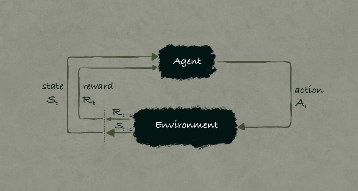
At the heart of reinforcement learning is the interaction between an agent (our chess-playing AI) and its environment (the chess game). This interaction happens in discrete time steps and follows a specific pattern:
The agent observes the current state (S₁) - in chess, this is the current board position
Based on this state, the agent selects an action (A₁) - a specific chess move
The environment responds with:
A new state (S₂) - the new board position after both players move
A reward (R₂) - perhaps +1 for capturing a piece, -1 for losing one, or +100 for checkmate
This cycle continues, creating a sequence: S₁, A₁, R₂, S₂, A₂, R₃, S₃, ... and so on.
The Mathematical Framework: Markov Decision Processes (MDPs)
This interaction is formalized as a Markov Decision Process (MDP), which has five key components:
A set of states (S) - all possible chess board configurations
A set of actions (A) - all legal chess moves
A set of rewards (R) - numerical feedback values
State transition probabilities - how likely each new state is, given the current state and action
Reward probabilities - how likely each reward is, given the state and action
In a finite MDP, these sets contain a finite number of elements, making the problem mathematically tractable.
The Dynamics Function
The environment's behaviour is completely described by the dynamics function:
$$p(s', r | s, a) = \Pr\{S_t = s', R_t = r | S_{t-1} = s, A_{t-1} = a\}$$
This function gives the probability of transitioning to state s' and receiving reward r, given that we were in state s and took action a.
Let's break this down with our chess example:
s: Current board position with your knight threatened by an opponent's pawn
a: Move your knight to safety
s': New board position after your move and your opponent's response
r: Reward (perhaps +0.5 for saving your piece)
The dynamics function tells us the probability of ending up in state s' with reward r after taking action a in state s.
The Markov Property
A critical aspect of MDPs is the Markov property, which states that the future depends only on the present state and action, not on the history of how we got there. In chess terms, the best move depends only on the current board position, not on the sequence of moves that created it.
This might seem counterintuitive at first - doesn't chess strategy depend on understanding your opponent's past moves? The key insight is that if the "state" is properly defined to include all relevant information (perhaps including a model of your opponent's strategy based on their past moves), then the Markov property holds.
Derived Quantities from the Dynamics Function
From the dynamics function, we can derive other useful quantities:
- State-transition probabilities:
$$p(s' | s, a) = \sum_r p(s', r | s, a)$$
- Expected rewards for state-action pairs:
$$r(s, a) = \sum_r r \sum_{s'} p(s', r | s, a)$$
- Expected rewards for state-action-next-state triples:
$$r(s, a, s') = \sum_r r \left[ \frac{p(s', r | s, a)}{p(s' | s, a)} \right]$$
The Agent-Environment Boundary
An important conceptual point is where to draw the line between agent and environment. In our chess example, the agent is the decision-making algorithm, while the environment includes the chess board, pieces, rules, and opponent.
The general principle is: anything the agent cannot arbitrarily change is part of the environment. The agent's knowledge about the environment is separate from this boundary - an agent might know everything about chess rules but still face a challenging learning problem.
2. Goals and Rewards
In reinforcement learning, the agent's goal is formalized through rewards - numerical values that the agent receives after each action. The fundamental principle is the reward hypothesis:
All goals can be described as the maximization of expected cumulative reward.
Designing Reward Signals
Designing an effective reward signal is crucial but tricky. For our chess AI:
Too sparse: Only +1 for winning, -1 for losing, 0 otherwise. This makes learning slow because feedback is delayed until the end of a long game.
Too frequent/misleading: +1 for each piece captured might encourage the AI to sacrifice important pieces to capture pawns.
Well-designed: Perhaps +0.1 for controlling center squares, +0.5 for checking the opponent, +1 for capturing pieces (weighted by value), and +100 for checkmate.
The key principle is that rewards communicate WHAT to achieve, not HOW to achieve it. If we reward subgoals too strongly, the agent might optimize for those at the expense of the true goal.
For example, if we heavily reward capturing pieces, our chess AI might sacrifice positional advantage just to capture a pawn. Instead, the reward should reflect the true objective - winning the game - with smaller rewards for actions that generally contribute to that goal.
Examples of Reward Design
Chess AI: +100 for checkmate, -100 for being checkmated, +piece_value for captures, -piece_value for losses, small rewards for controlling important squares.
Robot Navigation: -1 for each time step (to encourage efficiency), -10 for collisions, +100 for reaching the goal.
Stock Trading Agent: Reward proportional to portfolio value increase, with perhaps small penalties for excessive trading (to discourage churn).
The art of reward design involves balancing immediate feedback (to guide learning) with alignment to the true objective (to ensure the right behavior is learned).
3. Returns and Episodes
Now that we've defined states, actions, and rewards, we need to formalize the agent's objective: maximizing the expected return. The return is the function of future rewards that the agent aims to maximize.
Episodic Tasks
In episodic tasks, the agent-environment interaction naturally breaks into distinct episodes with clear endpoints. A chess game is a perfect example - each game starts from the initial board position and ends with checkmate, stalemate, or resignation.
For episodic tasks, we define the return as the sum of rewards from the current time step until the end of the episode:
$$G_t = R_{t+1} + R_{t+2} + R_{t+3} + \dots + R_T$$
Where T is the final time step of the episode.
For our chess AI, this would be the sum of all rewards received from the current position until the game ends.
Continuing Tasks
In continuing tasks, the interaction continues without a natural endpoint. Examples include ongoing process control or a robot that operates continuously.
For these tasks, summing rewards could lead to infinite returns, making it impossible to compare policies. To solve this, we introduce discounting:
$$G_t = R_{t+1} + \gamma R_{t+2} + \gamma^2 R_{t+3} + \dots = \sum_{k=0}^\infty \gamma^k R_{t+k+1}$$
Where γ is the discount rate (0 ≤ γ ≤ 1).
The Discount Rate
The discount rate γ determines how much the agent values future rewards:
γ = 0: "Myopic" agent that only cares about immediate rewards
γ close to 0: Agent values near-term rewards much more than long-term rewards
γ close to 1: Agent values future rewards almost as much as immediate ones
In chess, a low γ might lead to an agent that greedily captures pieces without considering long-term positional disadvantages. A high γ would encourage strategic play, where the agent might sacrifice material for long-term advantage.
Recursive Relationship of Returns
Returns at successive time steps are related recursively:
$$G_t = R_{t+1} + \gamma G_{t+1}$$
This recursive relationship is fundamental to many RL algorithms and helps us understand how value propagates backward from future states to current states.
4. Unified Notation for Episodic and Continuing Tasks
To handle both episodic and continuing tasks with a single notation, we use a clever mathematical trick: we treat episode termination as entering a special absorbing state that transitions only to itself and generates only rewards of zero.
This allows us to use the discounted return formula for both types of tasks:
$$G_t = \sum_{k=0}^\infty \gamma^k R_{t+k+1}$$
For episodic tasks, we can either:
Set γ = 1 and rely on the episode's finite length
Use γ < 1 and treat the terminal state as absorbing with zero rewards
This unified notation simplifies our mathematical framework and allows us to develop algorithms that work for both types of tasks.
5. Policies and Value Functions
Policies
A policy (π) defines the agent's behavior - it's the strategy that maps states to actions. In reinforcement learning, we typically use stochastic policies, where π(a|s) gives the probability of taking action a in state s.
For our chess AI, the policy would specify the probability of making each possible move in any given board position. A deterministic policy would always choose the same move in the same position, while a stochastic policy might sometimes explore different options.
Value Functions
Value functions estimate how good it is for the agent to be in a given state (or to take a given action in a given state). They're defined in terms of expected future returns.
State-Value Function
The state-value function for policy π is defined as:
$$v_\pi(s) = \mathbb{E}\pi[G_t | S_t = s] = \mathbb{E}\pi\left[\sum_{k=0}^\infty \gamma^k R_{t+k+1} | S_t = s\right]$$
This gives the expected return when starting in state s and following policy π thereafter.
In chess terms, vπ(s) would tell us the expected outcome (in terms of our reward metric) when starting from board position s and playing according to strategy π.
Action-Value Function
The action-value function for policy π is defined as:
$$q_\pi(s, a) = \mathbb{E}\pi[G_t | S_t = s, A_t = a] = \mathbb{E}\pi\left[\sum_{k=0}^\infty \gamma^k R_{t+k+1} | S_t = s, A_t = a\right]$$
This gives the expected return when starting in state s, taking action a, and thereafter following policy π.
In chess, qπ(s, a) would tell us the expected outcome when making a specific move a from position s, and then continuing with strategy π.
The Bellman Equation
A fundamental property of value functions is that they satisfy recursive relationships known as Bellman equations. For the state-value function:
$$v_\pi(s) = \sum_a \pi(a|s) \sum_{s', r} p(s', r|s, a)[r + \gamma v_\pi(s')]$$
This equation expresses a relationship between the value of a state and the values of its successor states. It's saying that the value of the current state equals the expected immediate reward plus the discounted value of the next state.
In chess terms, the value of a position equals the immediate benefit of your next move (capturing a piece, controlling the center, etc.) plus the discounted value of the resulting position.
Backup Diagrams
Backup diagrams visually represent these recursive relationships. They show how value information "backs up" from future states to the current state.
For the state-value function, the backup diagram shows:
The current state at the top
Actions available from that state
Possible next states resulting from each action
The value backing up from those next states to the current state
These diagrams help visualise the flow of value information in reinforcement learning algorithms.

6. Optimal Policies and Optimal Value Functions
The goal in reinforcement learning is to find an optimal policy - one that achieves the maximum expected return from all states. This leads us to define optimal value functions.
Optimal State-Value Function
The optimal state-value function, v*(s), gives the maximum value achievable by any policy for each state s:
$$v_*(s) = \max_\pi v_\pi(s)$$
In chess, v*(s) would tell us the expected outcome when playing optimally from position s.
Optimal Action-Value Function
Similarly, the optimal action-value function, q*(s, a), gives the maximum expected return for each state-action pair:
$$q_*(s, a) = \max_\pi q_\pi(s, a)$$
In chess, q*(s, a) would tell us the expected outcome when making move a from position s and then playing optimally thereafter.
Bellman Optimality Equations
The optimal value functions satisfy special Bellman equations called Bellman optimality equations:
$$v_(s) = \max_a \sum_{s', r} p(s', r|s, a)[r + \gamma v_(s')]$$
$$q_(s, a) = \sum_{s', r} p(s', r|s, a)\left[r + \gamma \max_{a'} q_(s', a')\right]$$
These equations express the principle that the value of a state under an optimal policy equals the expected return for the best action from that state.
Finding Optimal Policies
Once we have the optimal value functions, finding an optimal policy is straightforward:
With v*: Choose actions that maximize the expected value of the next state
With q*: Simply choose the action with the highest q*(s, a) in each state
This is why q* is particularly useful - it directly tells us which actions are best in each state without requiring additional computation.
Greedy Policies
A policy that always selects the action with the highest estimated value is called a greedy policy. When we have the true optimal value function v*, a greedy policy with respect to v* is guaranteed to be optimal.
In chess, this would mean always making the move that leads to the position with the highest v* value.
7. Optimality and Approximation
While we've defined optimal policies and value functions mathematically, finding them exactly is often computationally infeasible for real-world problems.
Computational Challenges
For many interesting problems, the state space is enormous:
Chess has approximately 10^43 legal positions
Go has approximately 10^170
Real-world robotics problems have continuous state spaces with infinite states
Even with today's computing power, we cannot solve the Bellman optimality equations exactly for such large problems.
The Role of Approximation
In practice, reinforcement learning relies on approximation methods:
Function approximation: Using parameterized functions (like neural networks) to represent value functions
Sample-based learning: Learning from experience rather than complete knowledge of the environment
Temporal difference learning: Bootstrapping estimates from other estimates
Focusing on Important States
A key advantage of reinforcement learning is that it can focus computational resources on states that the agent actually encounters, rather than trying to learn optimal behavior for all possible states.
In chess, professional players don't memorize optimal moves for all 10^43 positions - they focus on positions that commonly arise in games. Similarly, reinforcement learning algorithms can prioritize learning about frequently encountered states.
Balancing Exploration and Exploitation
A fundamental challenge in reinforcement learning is the exploration-exploitation dilemma:
Exploitation: Using current knowledge to maximize rewards
Exploration: Trying new actions to discover potentially better strategies
In chess, this would be like deciding whether to play a familiar opening (exploitation) or try a new one (exploration).